A couple of years ago, I was part of a group that published a method on calculating body mass in extinct animals from laser scans of their skeletons. The method involves separating the model into parts, and then using the qhull command to produce a volume that encloses the segment as tightly as possible. This in turn gives you a minimum volume, and as animals have an average density a bit lower than water, you can get a mass.
However, the method involves using Matlab, which is not free (though is generaly available through institutions to academics), and also involves what I consider some finickety file handling as you chop up models and reassemble them.
So, here I’ll show you how it can now all be done in Meshlab (one of my free software faves), from importing your skeleton, to getting a volume estimate (which is then used to calculate mass).
Step 1, get a model of the skeleton.
If you don’t have one to hand, but want to follow along, I have several skeletons available with various publications (though admittedly none are dinosaurs):
From the Manchester Museum, and associated with my Palaeontologia Electronica Paper in 2012 on photogrammetry. (note that PE just provide all the models as a single zip, so you’ll also get a trilobite, a trackway, and a tree!)
-or-
From the Brown University teaching collection, my 2013 JPT paper on using the Microsoft Kinect to scan fossils.
(If you use either of these models in your work, please cite the respective papers).
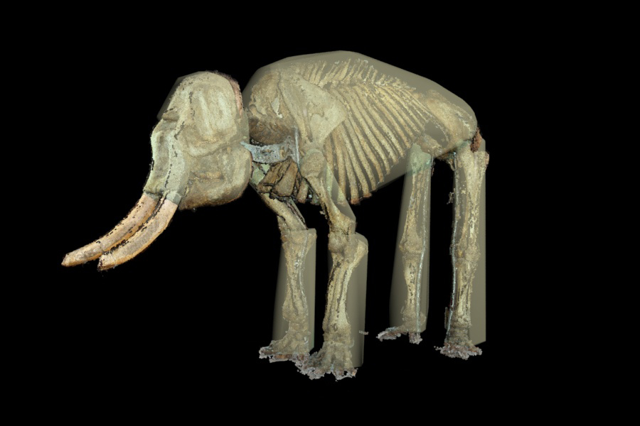
I’m going to use the elephant, as it’s a while since I’ve played with that model.
If you want to use your own, it’s dead easy to get a model using photogrammetry, and there are plenty of guides available (such as mine, available here, or Mallison and Wings’ JPT article here).

Here it is. When I created the model, I did scale it, so we at least don’t have to worry about that, but looking at the model now I see I was a bit naughty in not cleaning up the extraneous points – there are some around particularly the forelimbs, and there are some ridges caused by alignment issues on top of the tusks and the front of the skull, so let’s clean those up.
Step 1b – cleaning the model (if your model is clean, skip ahead!)
To remove the points near the feet, rotate the model so we’re looking at the feet, and the floor is straight. This lets us select all those points with the rectangle tool, and delete them all in one go:

We’ll be using these tools a lot, so make note of where they are. (If you have a meshed skeleton, like the pronghorn, you need the ‘delete triangles’ button next to the ‘delete selected points button’)
To get rid of the points on the tusks, I’ll show you a neat little trick I often use. You’ll notice that those points are black (the colour of the museum background at the time), but all the bits we’re interested in are, well, bone coloured. Head to Filters->Selection->Select faces by colour (or, ‘color’ as meshlab insists on Americanisms). Make sure the ‘preview’ check box is ticked. Click on the colour box and pick a colour close to the colour of the points on the tusks you want to get rid of – in this case fairly grey. I prefer to work in RGB, but if you can work in HSV go for it. Then alter the sliders until it looks like you have most of the points you want to get rid of. It might look like you’re getting rid of a lot, but as convex hulling only requires the extreme limits of segments, it doesn’t matter too much. Once selected, hit apply, then delete the points. This method is great when the geometry doesn’t allow simple rectangular selections.

Pro-tip: When selecting the colour, there’s actually a button called pick screen colour, which you can use to directly click on a point you want to get rid of to select its colour specifically.
Having cleaned the model, it’s time to start separating the bits out.
Step 2: Split the model into sensible parts.
Convex hulling works by enclosing a set of points (or a mesh) without any inward pointing parts. So if we hulled the model as it stands, this would be the result:

Clearly, this is not elephant-like, and considerably over estimates the volume. So we’re going to break the model up into the individual legs, the torso, the head, and the tusks. With dinosaurs, you would also separate out the tail – the goal is to get a series of convex hulls that enclose the bones as tightly as reasonable.
Firstly, we want to make our layers pane visible, by pressing the ‘layers’ button. Next, we start selecting parts of the model as best we can with the select tool we used earlier on the floor. Select one leg, as best as you can without getting much pelvis. In this model, I still have the metal supports next to the hind limbs, and you should really get rid of those, but it doesn’t matter too much here. Select as much as you can, then hit the selection button to move the model around to get a better view of any points you couldn’t select before. Then go into selection mode again, and you can hold ctrl or shift to add or remove points from your selection. When you’ve got a selection you’re happy with, like below, right click on the model in the layers pane, and select ‘move selected vertices to another layer’ – if you’re using a meshed skeleton, you’ll want move selected triangles. I like to delete the original selection each time, so my last segment doesn’t need doing specifically.

Now we have one layer for the rear left leg, and one layer with everything else. Repeat for each segment. I find it helps to click the eye icon for each new layer to turn it off and make it clear what you’ve got left. Here, I’ve coloured each part separately so you can see how I’ve divided the model.

I’ve left the tusks separate – let’s not include those in our mass estimate as tusks are weird external features that don’t really have soft tissue for us to model. You might want to separate the feet, or the pelvis…. That’s your call to make depending on how you consider the convex hull fits the parts.
Step 3: Convex hulling
Now it’s time to convex hull each part of our model. Work down the layers list (the selected layer will be highlighted in yellow), and for each layer go to Filters->Remeshing, Simplification, and Reconstruction->Convex Hull. Tick ‘Re-orient all faces coherently’ to make the hull have correct normals, and hit apply.

If the hull looks dark, head up to Filters->Normals, Curvature, and Orientation->Invert Faces Orientation, and hit apply. This should make the hull look ligher, because now the faces are oriented pointing outwards.

As I hull each part, I like to turn off visibility for the skeleton part I just hulled. It keeps everything nice and clean and easy to tell what you’ve done or not done. You can also move to each layer without closing the convex hull dialogue box, or press Ctrl+P to repeat the last command on the layer you have selected. Eventually, you will have hulled the entire thing, and you’ll be left with a very blocky looking animal:

I’ve left the tusks in the image to orient you a bit better.
Part 4: Getting the hull volume.
Now we’re on the finishing straight. Make sure all your skeleton layers are turned off, and all your convex hulls are turned on. Right click in the layers section and choose ‘Flatten Visible Layers’ (you may want to save each convex hull separately first depending on what you want to do later!). This will merge all the hulls into a single mesh. Now go to Filters->Quality Measure and Computations->Compute Geometric Measures. In the bottom right, beneath the layers pane, are the measures for the convex hull. We’re interested here in ‘Mesh Volume’ (you may have to scroll up a little) – I’m getting 2.65295 cubic meters (a small note – small models may need scaling up, or scaling in cm, as Meshlab only shows six decimal places, see here). Note also that the centre of mass is reported down here too, which you may be interested in.
What happens now depends on how detailed you want to get. My colleagues and I tend to create airsacs based on anatomy, and subtract these from the volume, but let’s not get into that here. Instead, let’s just apply a bulk density for the animal. Sellers et al 2012, where we first published the convex hulling method, refer to a total bulk density for horses of 893.36 kg/m3, so let’s use that to multiply our volume:
2.65295 m3 * 893.36 kg/m3 = 2370.04 kg.
This is our minimum mass for the elephant, but Sellers et al suggested that the minimum convex hull underestimated mass by about 21% over the range of animals they used. That would give us a value of 2867.75 kg, or just shy of 3 tonnes. Now unfortunately, I don’t have the mass data for this animal before it became a mounted skeleton in the Manchester Museum, but Wikipedia tells me the average weight for females is 2.72 t, with males getting up to 5.4 t, so we’re definitely in the right ball park. Measuring up the elephant (using the measure tool in meshlab), I get about 2.4 m high, so not a particularly large male – infact about the same size as Wikipedia tells me those 2.72 t females are.
So we’re pretty close there. I haven’t actually used this method over the old Matlab one for a publication yet, so if you spot any glaring errors, I’d be happy to hear them.
Part 5: the wrap up.
This was obviously a really quick and dirty run through, and we just threw a bulk density in there instead of modelling lungs and the like, so I’m not claiming this is bullet proof. And it’s worth noting that there a whole bunch of caveats to using this method, especially on extinct animals about which we just don’t know exactly what density they might have been. But it is a great way of quickly getting a minimum possible mass.
Here’s my final convex hull + skeleton rendered in 3d studio Max:

I hope this was either useful or interesting. If this is useful to your own work, please cite the Sellers et al paper (unless you can cite blog posts like this directly, in which case do that too):
Sellers WI, Hepworth-Bell J, Falkingham PL, Bates KT, Brassey Ca, et al. (2012) Minimum convex hull mass estimations of complete mounted skeletons. Biology Letters 8: 842-845.
Also, cite meshlab accordingly.
